Sampling Methods within TensorFlow Input Functions

Many real-world machine learning applications require generative or reductive sampling of data. At training time this may be to deal with class imbalance (e.g. rarity of positives in a binary classification problem, or a sparse user-item interaction matrix) or to augment the data stored on file; it may simply be a matter of efficiency.

In this post, we explore some sampling techniques in the context of propensity modelling and recommender systems, using tools available in the tf.data API, and present which methods are beneficial with given data and hardware demands.

Naïvely, a precomputed subsample of data will make for a fast input function. But to take advantage of random samples, more must be done. We first consider how to select from a large dataset containing all possible inputs. Conversely, we look at generating these in memory using tf.random and exploiting HashTables where appropriate. As a side effect, these methods grant additional flexibility to the user and reduce data preparation workloads.

We’ve developed a TensorFlow sampling module coupled with two real-world examples, you can find the code on GitHub. We also presented this work at the O’Reilly TensorFlow World conference in Santa Clara (October 2019) and you can find the presentation here.

Why sample?

Dataset distributions

In supervised learning problems, we care about the relationship between inputs X and outputs Y. The distribution of examples is normally a secondary concern, but can be worth a moment’s thought. In general, a dataset may overrepresent certain regions of the X or Y domain compared to the real process, and the choice of what we train a model with may be different again.

An uneven sample of X and Y does not affect the nature of the implicit function linking them. However, it very much affects the learning procedure when approximating that function. One of the prerogative powers of an ML practitioner is being able to alter the distribution of learning examples to create an ideal learning environment.

How sampling affects the learning process

Even though the learned function will, in theory, be no different just because the data distribution changes (as long as the training examples carry enough information), a non-ideal learning setup can be unhelpfully slow to learn in. Ideality is achieved at high entropy, i.e. more uniform distributions of X and Y. For example, in a binary classification problem we want equal quantities of the positive and negative label to learn from.

Why? Because to learn where the function changes, we need data spanning these changes. An update based solely on one class will not tell us anything about where a class boundary is, only where it is not. And since iterative model-adapting procedures (like training a neural network through stochastic gradient descent) are not well-equipped to retain knowledge of where a class boundary isn’t, we prefer to see evidence of where it is and update our estimate accordingly. Otherwise, we can spend a lot of time making poor-quality updates.

Side-effects of sampling

Sampling from a dataset is a way of altering the distribution of examples. Often the goal is to make this distribution more uniform (as discussed in the previous section). There are a few side-effects to consider, though:

• Fewer examples ⇒ poorer signal–noise ratio

By discarding data, information is lost. The uncertainty in the solution increases, although this effect may be minimal as it also depends on the statistics of the dataset. In the worst case, the quality of the learned model will suffer, and it also makes overfitting a more prominent risk.

• More examples ⇒ more computation

Every piece of training data brings with it corresponding storage, processing, transfer and modelling computation needs. This adds time and expense, as well as potentially complicating engineering pipelines.

• Different distribution ⇒ different output probabilities

A subtle point, but any probabilistic interpretation of the model is conditioned on the dataset used to train it. These will not accurately reflect real-world probabilities if the distributions are different.

Weighting

As an alternative to sampling (binary inclusion or exclusion from the dataset), we can ascribe different sample weight to different regions of the input space.

This is often as simple as scaling the gradient update step so that certain regions have more of an impact towards training than others. It may be appropriate to weight instead of sampling, so as to retain all the signal in the dataset without discarding any. But it is perfectly reasonable to sample and weight simultaneously, to achieve benefits from each technique. Again, the nature of the learned solution should not change – all we are altering is the statistics of the learning process. For example, the following learning environments for a binary classification give equivalent solutions:

Further reading

Some other techniques for working with imbalanced data include

• Cost-sensitive models or loss functions, where the weighting is applied when calculating the loss, rather than applying a gradient update. 
• Data augmentation techniques e.g. SMOTE, where examples are interpolated smoothly to generate fake data from a similar distribution.
• Imbalance-robust algorithms, where the learning is less adversely affected by low-entropy training data than NNs are.

tf.data and tf.estimator APIs

tf.data > queues > feed_dict

Before the introduction of the tf.data module, the way in which data was fed into the TensorFlow graph for model training was through the feed_dict or Queues mechanism.

feed_dict is a way of pulling the input processing outside TensorFlow and into the Python program itself. As the name suggests, feed_dict  is just a dictionary that maps graph elements to values – placeholders are declared with tf.placeholder, and the actual values are specified with thefeed_dict argument when running a TensorFlow session. This works fine for small datasets that fit in-memory, but performance-wise it can be suboptimal. One of the reasons is because feed_dict is an example of a synchronous implementation where you often run processing in a single thread and on the critical path, such that data being loaded and processed on the CPU leaves the accelerator sitting idle, and the accelerator training a batch of data leaves the CPU sitting idle. 

This is where Queues come into the picture.Queues give us memory optimisation, asynchronicity and multi-threading properties. But TensorFlow developers wanted to create an API more performant than both feed_dict and Queues , and much easier to use.

tf.data or the Dataset API was introduced as a core module in TensorFlow version 1.4, and was presented as the recommended way to build flexible and efficient data input pipelines to TensorFlow models.

TensorFlow input pipelines can be described as a standard ETL process:

• Extract – ability to create a Dataset object from in-memory or out-of-memory datasets using methods such as:
  • tf.data.Dataset.from_tensor_slices – if your dataset is in-memory
  • tf.data.Dataset.from_generator – if elements are generated by a function
  • tf.data.TFRecordDataset – if your data is in the serialised TFRecord format
  • tf.data.TextLineDataset – if your data is in the form of text files
• Transform – transforming the Dataset by applying preprocessing operations such as:
  • tf.data.Dataset.batch – stacks together multiple consecutive elements to form batches
  • tf.data.Dataset.shuffle – randomly shuffles the elements in a buffer
  • tf.data.Dataset.map – applies a function to each element
  • tf.data.Dataset.repeat – repeating the Dataset a certain number of times
• Load – loading batched examples onto the accelerator ready for processing. Elements can be prefetched asynchronously using the tf.data.Dataset.prefetch method, preventing the accelerator from data starvation.

The class diagram for Datasets is shown below, where the Dataset base class contains methods to create and transform datasets, and TextLineDataset, TFRecordDataset and  FixedLengthRecordDataset are subclasses. An Iterator can be instantiated in order to access elements one at a time.

Estimators

We have spoken about how to build input pipelines, but what about training a Machine Learning model? Estimators (tf.estimator) was introduced in TensorFlow version 1.3 as a high-level API that simplifies the Machine Learning process.

Before Estimators, the typical model development cycle involved a lot of boilerplate code to represent features, construct model layers, establish training and validation loops, distribute model training, so on and so forth. But the Estimator class has been designed to abstract a lot of this away, containing the necessary code to:

• run a training or evaluation loop
• predict using a trained model
• export a prediction model for use in production

The Estimators API enables us to build TensorFlow machine learning models in two ways:

1. Canned – “users who want to use common models”

1. • Common machine learning algorithms made accessible such as multilayer perceptron, wide and deep, and boosted trees
   • Robust with best practices encoded
   • A number of configuration options are exposed, including the ability to specify input structure using feature columns
   • Provide built-in evaluation metrics
   • Create summaries to be visualised in TensorBoard

2. Custom – “users who want to build custom machine learning models”

1. • Flexibility to implement innovative algorithms
   • Fine-grained control
   • Model function (model_fn) method that build graphs for train/evaluate/predict must be written anew (whereas this is already written for canned Estimators)
   • Model can be defined in Keras and converted into an Estimator (tf.keras.estimator.model_to_estimator)

The class diagram for Estimators is given below where Estimators is the base class and canned estimators are direct subclasses. As you can see, Estimators call an input function (input_fn) to retrieve the input pipeline.

Getting data from A to B

So far we have spoken about the input pipeline to read data into your program using Datasets, and how to define a Machine Learning model with Estimators. How do we connect the two together? Well, data for training, evaluation and prediction must be supplied through user-defined input functions, which acts as a wrapper for the set of Dataset operations. A valid input_fn takes no arguments, returning either a tuple (features, labels) or a Dataset generating such tuples to be used for the Machine Learning component:

• features – Tensor of features, or dictionary of Tensors keyed by feature name
• labels – Tensor of labels, or dictionary of labels keyed by label name

A new graph is generated whenever one of the train, evaluate and predict methods are called, and the input_fn produces the input pipeline of the Estimator, followed by model_fn being called to build the model graph.

Typically, an input function is structured as shown in the figure below, where a Dataset is instantiated by connecting to the source data, transformations are applied in sequence, and finally, an Iterator object is created over the Dataset  to manually retrieve batches of elements. The most common is the tf.data.Dataset.make_one_shot_iterator method which will yield elements until tf.errors.OutOfRangeError exception is thrown, and theDataset is exhausted. 

This is by no means a rigid structure – the input function can be designed to accept arguments like the data source paths, schema, and parameters for theDataset  transformation methods, enabling us to build input functions with variable settings. Also, the Dataset  can be returned for use with the Estimator without having to create an Iterator over it, the importance is on ensuring the Dataset  is comprised of (features, labels) pairs.

It is important to note that the order of transformations matter – ordering operations in a certain way can have performance implications. For example, a pipeline with the repeat operation followed by the shuffle operation will be performant, but there is no guarantee that all examples will be processed in an epoch. If we switch the order of these operations, then we have stronger ordering guarantees but it may not be as performant. Best practices around creating an efficient input pipeline are explained in detail in the TensorFlow documentation.

Putting it all together

Now that we’ve understood the purpose of an input function, let’s see how it fits in with the key stages of a simple modelling pipeline:

1.) Define input function for passing data to the model for training and evaluation

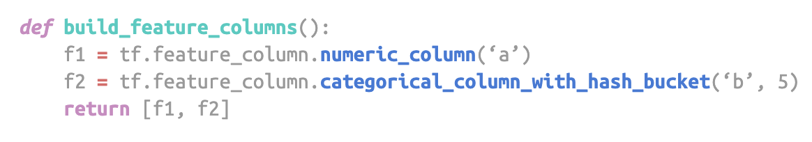
2.) Define feature columns which are specifications for how the model should interpret the input data

3.) Instantiate Estimator with necessary parameters and feeding in the feature columns

4.) Train and evaluate model – train loop saves model parameters as checkpoint, eval loop restores model and uses it to evaluate model

5.) Export trained model as SavedModel

6.) Evaluate model – compute evaluation metrics over test data

7.) Generate predictions with trained model

Sampling in behavioural modelling problems

At Datatonic, we often see datasets detailing how a user base interacts with products, interfaces or other items. Models built on such data might include propensity prediction or recommendation.

A useful feature of these datasets is that we construct each example to be a (user, item) pair. The matrix of possible pairs is typically highly imbalanced given that many (user, item) pairs are simply not observed, but, if input features are confined to user features and item features, they can at least be generated.

Pair generation in a tf.data pipeline

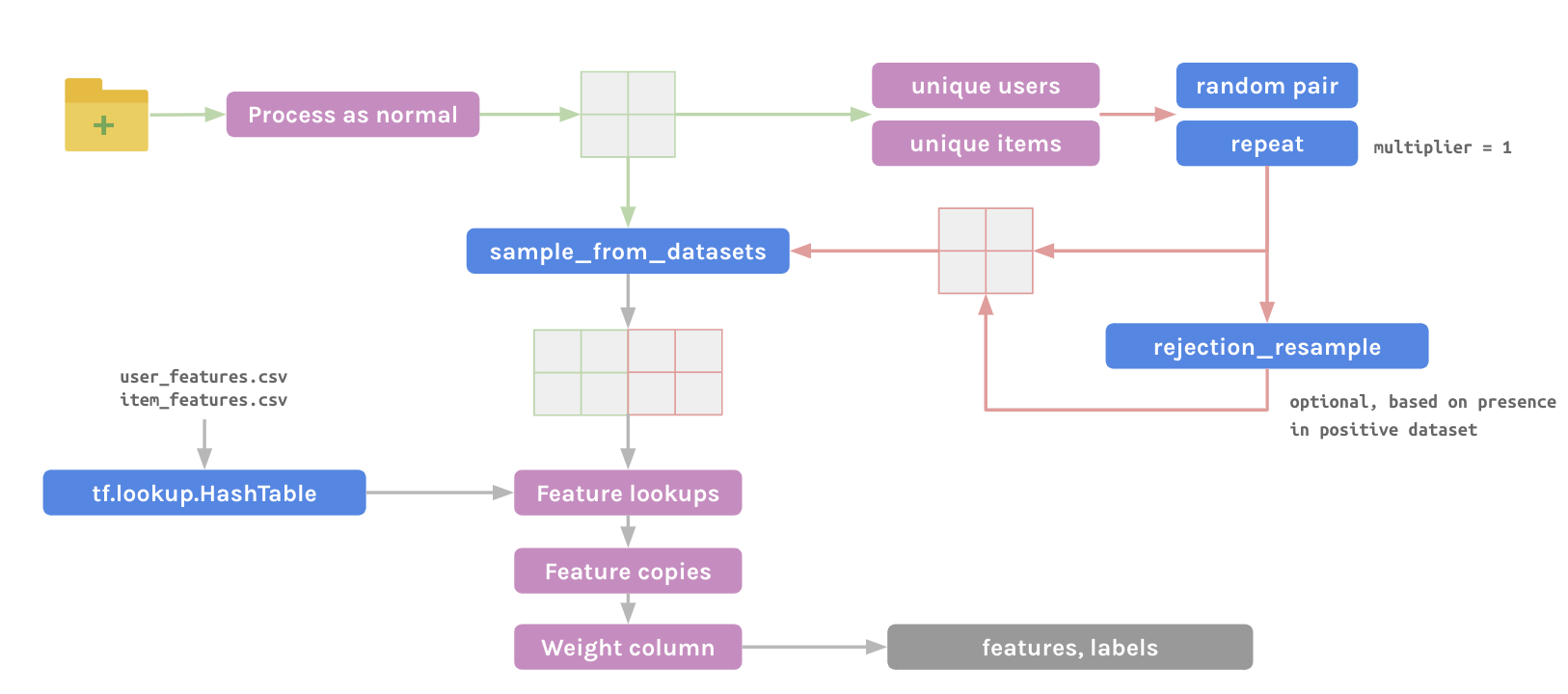
Completely avoiding any storage or file reading of negative examples, this technique centres on generating random (user, item) pairs to form the negative dataset. Cached information (a user list, item list, and associated features) is exploited to make this a very efficient pipeline.

Using sampling tools inside TensorFlow, each negative example generated can be checked for novelty against the positive dataset (though this is one of the slowest steps and not strictly needed), then combined randomly with positive examples to form a mixed overall dataset. HashTables are convenient for the rejection resampling and feature lookups.

Take a look at our implementation of this method for a recommender systems problem using the Million Songs dataset.

Downsampling and upweighting in tf.datapipeline

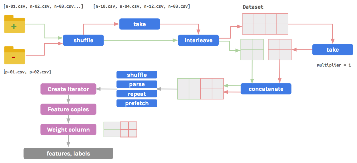
An effective way to handle imbalanced data is to downsample and upweight the majority class:

• Downsample – extract random samples from the majority class known as “random majority undersampling”

• Upweight – add a weighting to the downsampled examples (weight should typically equal the factor used to downsample)

There are several benefits for applying such a method. The model will converge faster as the minority class will be seen more often during training. Upweighting the majority class (following downsampling) will ensure the model outputs are calibrated and interpretable as probabilities. Consolidating the majority class into fewer examples requires less processing of data. A significant disadvantage of this method is that it discards a portion of available data, however modifications can be introduced in the downsampling process to overcome this shortcoming.

This technique assumes a separation of positive (minority) and negative (majority) examples. The list of files are themselves shuffled before a subset of files containing the negative examples is selected. Dataset objects are created for both sets of examples. The negative Dataset is randomly downsampled based on a user-supplied multiplier, and concatenated with the positive Dataset. After a series of transformations are applied, a weight column is dynamically generated by mapping the label column to a user-supplied weight.

Take a look at our implementation of this method for a propensity modelling use case on the Acquire Valued Shoppers dataset.

Summary

In this post we walked you through the rationale behind why sampling can be effective in Machine Learning workflows, followed by an introduction to building efficient input pipelines for Machine Learning models using the TensorFlow tf.data and tf.estimator APIs, and finally two custom methods for sampling directly inside input functions.

The sampling module we’ve developed along with two real-world examples can be found on GitHub.